Conceptual Site Model for a Contaminated Industrial Area in Marche Region, Italy

CHARACTERIZATION SITE

Geographic Localization:

The study area that is taking into account for the project is the “API Raffineria di Ancona” area in Falconara Marittima, province of Ancona, Marche region on the Adriatic coast of Italy.

This area is bordered to the northeast by Adriatic Sea, by the Esino River to the northwest and by another property of API and the highway to the south.

Site Geological and hydro-geological structure:

The low valley of the river is located in the last part of the Basin, which was born in the Early-medium Miocene.

The main types of rocks present in the valley of the river are partially cemented sandstone, calcium sulphate, clayed loam, alternation of sandstone, loamy clay and thin layer silty sand.

Mountain chain typical characteristics can be easily recognized in the area, with folds and faults in the direction of E-W.

The main structures were determined by tectonic event in the medium Pliocene. It caused the uplift of the most part of the area. During the passage Pliocene-Pleistocene a marine ingression determined a progressive uplift of the area. Initially the marine sedimentation proceeded in the western part while the eastern part raised; a group of fault in the low zone of the valley and NS oriented coincides with these two zones separation area.

There are also two groups of secondary faults: one is E-W oriented, the other has an ENE-WSW direction and is present in the Western part respect to the master fault. Some morphological hints say that during the period between low Pleistocene and medium Pleistocene there had been transcurrent movements along these faults.

Geomorphology:

The river originates from two sources and its flow direction depends on the tectonic orientation (N-S). The river channel is almost linear but it becomes “braided” close to the river mouth. It flows the right part of the alluvial plain without touching the central part, so that in the left part of the plain, were the erosion is less important, there are large alluvial terracing deposits while in the right part there are only the two more recent

Hydrogeology:

Groundwater is contained into the terracing alluvial deposits, mainly composed by gravel and sandy gravel.

The alluvial area is about 140 km2, the medium effective porosity is about 20% and the hydraulic conductivity values are between 6,5·10-4 and 2·10-3 m/s.

The aquifer is locally confined toward the sea due to the presence of thick clay-silty layers, so that it has the feature of a multi-layered one while is unique in the upper part.

The annual piezometric level range is about two meters and the groundwater presents its maximum level during the spring and the minimum in the autumn. The recharge is mainly due to rains and confluent channels. The groundwater is affected by the maximum rain with a delay of two months and it reaches its maximum after 8-9 months after the rain event.

Calcium carbonate is present in groundwater (especially in the recent terracing) while toward the coastline water is also rich in Mg and SO2-4.

Existing industrial activities currently or in past and considering chemical substances:

The site has been occupied since 1950 by refinery and storage of oil and petroleum products, and it is still being used for the same purposes. Excesses of crude oil, distillation products, gasoline, diesel fuel, kerosene and other petroleum substances are present at the site. Chemical additives present include MTBE octane enhancement, the fuel dyes GREENFARMING 01 and GREENECOL 02, and the corrosion controller CORTROL OS 7780. Other chemicals on site used for processing or created as byproducts include oxygen, hydrogen, nickel dust, hydrogen sulfide, carbon monoxide, and catalysts.

Available data for the study area:

Chemical analysis of soil

Chemical analysis of water

Chemical tests on the free phase

Bore-hole and location of wells

To emphasize the occurrence of two aquifers, the layers with lower permeability, which contain clays and silts, are considered using measurements of the piezometric level in the wells screened at different depths.

BACKGROUND:

Stratigraphy:

In the low valley of the river is possible to find, starting from the deepest part, the following rocks types:

Partially cemented sandstone, clayed loam, calcium sulphate and loamy clay (mesinian);

Alternation of sandstone, loamy clay and conglomerate levels on the base and then loamy clay with arenaceo levels (Early Pleistocene);

loamy clay with little lenses and very thin layers (a few millimeters) of silty sand (Middle Pleistocene).

The little sandstone and silty-sand layers don't have much influence on water circulation in the alluvial aquifers, whereas the last type in the list above is considered the impermeable substratum of the aquifers.

The alluvial aquifers are distributed in five orders of terracing and are constituted by gravelly-sandy deposits where sand, silt and clay lenses and layers are present, often rich of vegetable substances.

Wells distribution in the site:

The wells were distributed in all directions. The density is due to the purpose they serve. Some wells were drilled in southern part of the site along the coast line to identify the presence of impermeable layers that can affect the flow path of the pollutant. The flow direction from north to south, as we are going to see later, the purposes of the monitoring wells in the northern side of the site were drilled to:

1) Identify whether there is a polluted flow of from upstream sources of the site.

2) Identify the presence of impermeable layers that can block the path of the pollutant.

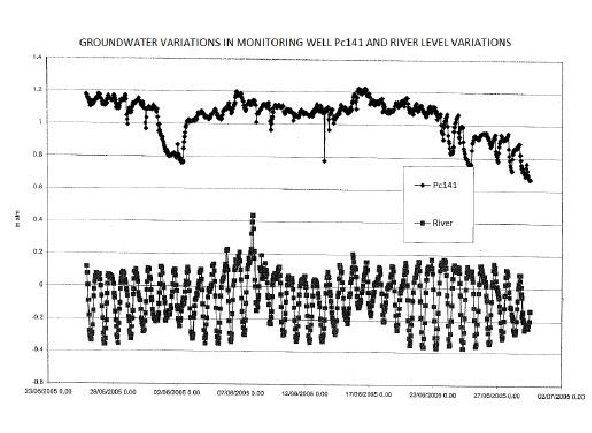
The wells in the eastern side of the storage tanks, parallel to the river, were drilled to measure the piezometric levels to understand the direction of the discharge. The piezometric level of well Pc141, shown in the Figure 3 below, shows groundwater level always higher than in the river, meaning that the polluted plume is discharged in the river.

The monitoring wells in the western side of the storage tanks were drilled for the same purposes of the wells in the northern direction, but they were successful in identifying the presence of a second acquifier. From the stratigraphies of the site, we observe that two monitoring wells located close to each other have different piezometric levels, PM7 and PS7.

The monitoring wells PM7, PS7, PM5 are closely located to each other, they have similar stratigraphies, where an impermeable layer of clay was detected in all of them at depth of 10 meters, but the confined aquifer was detected in the well PM7 and PM5 at depth of 25 – 30 meters.

Cross-sections:

In this site we created five cross-sections to identify the permeable and impermeable layers and their continuity, in addition to investigate the extension of the two acquifiers along the site to the sea and to the river. There are three cross-sections were parallel to each other and parallel to the coast line, A-A’, B-B’ and D-D’. Another cross-section is parallel to the river L-L’ and another one in the north-west part of the site and west direction of the storage tanks E-E’.

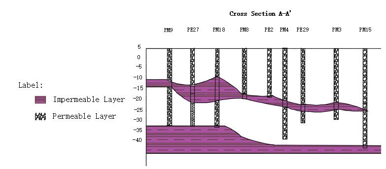
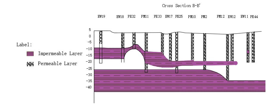
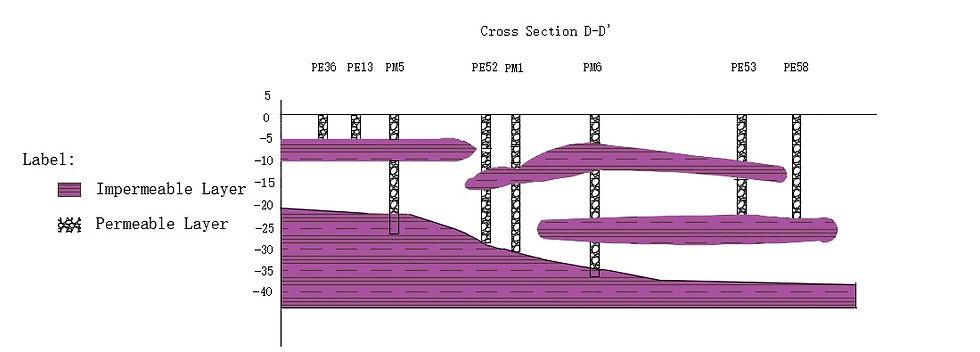
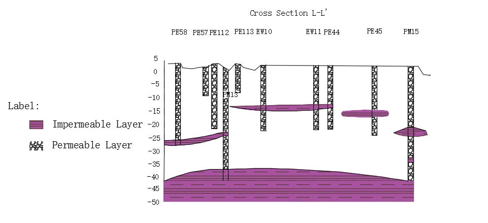
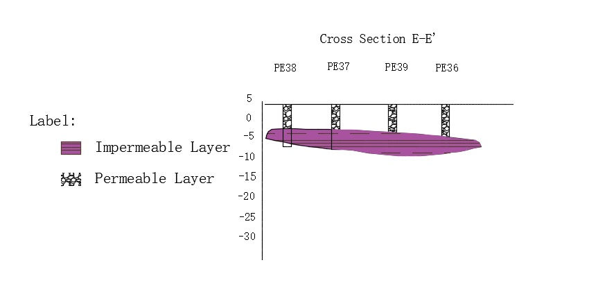
From the cross-sections we observed that the thick layer of clay that separates the two aquifers disappears as we move toward the sea or toward the river, causing the contamination of the second aquifer. The rock type of the first aquifer is a sandy-gravel, whereas the rock type of the second aquifer is sandy-gravel and the base layer is clay.

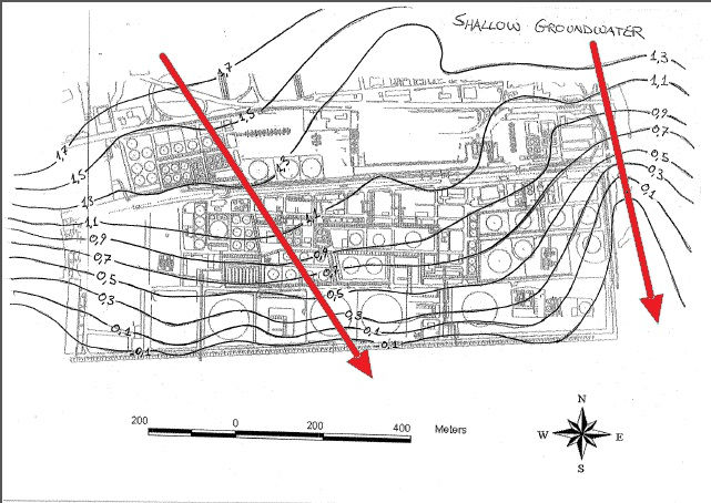
Flow direction:

The piezometric lines were obtained from the head values in the site, then the flow directions of the two aquifers. The flow direction is from north to south, which it is perpendicular to the piezometric lines.

LNAPL (Light Non-Aqueous Phase Liquid) CONTAMINANTS:

Contaminant sources:

Pollutants associated with petroleum products, additives present in the soil, or groundwater due to the industrial activities at the refinery site could be dangerous, so that it is needed to investigate their presence. They may have been introduced due to leaking of storage tanks at the site, and if so, remediation may be necessary.

Specialized monitoring and remediation plans for MTBE (Methyl tert-butyl ether), separate from the rest of the hydrocarbons present at the site, are required since its behavior in soil and groundwater is different from that of other hydrocarbons. MTBE has a higher solubility in water (up to 30 times more than benzene), lower propensity to adsorb to soil, and lower biodegradability than other hydrocarbons.

Definitions of the contaminants:

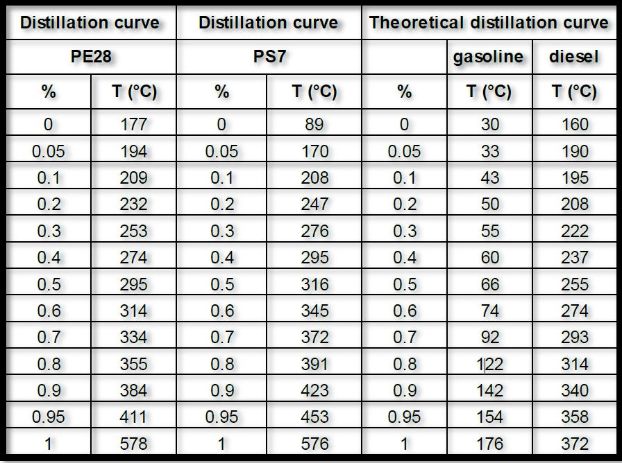
The nature of the contaminants can be quantified by plotting the distillation curve or boiling point composition curve Figure below. This curve is made by taking mixture contaminants compositions, heating them to the boiling point, measuring maximum temperature reached and analyzing the composition of the vapor above the mixture.

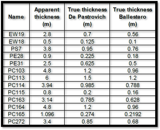
True LNAPL thickness and volume contaminants determination:

Generally, the presence of LNAPL contaminants might add complexity in characterization of the groundwater site because polluted liquids has densities less than water, thus the waste products float in the capillary fringe separately from the water table. Also, water level seasonal fluctuation affects LNAPLs thickness in a well (Wozmak, 2003). Thus, for the determination of contaminant’s volume in the study site we stated from the value of apparent thickness of LNAPLs in the different wells, and then we corrected the thickness using De Pastrovich and Ballestero formulas.

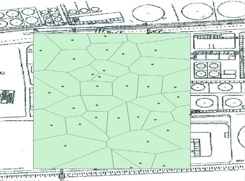
LNAPL volume valuation using Thiessen Polygons:

Determining volume of soil contaminant is an important step in the performance of site investigation, risk assessment and remediation. The volume can be estimated by determining the hydrocarbon concentrations in soil and hydrocarbon thickness in wells. The individual areas of influence of the contaminant in each well is determined with the Thiessen polygons. The boundaries of the polygons define the area that is closest to each well relative to all other wells.

The Thiessen Polygons were performed in the contaminated site, and the result is shown in Figure 13. Thereby the volume of contaminant was calculated by multiplying the area of influence of each well with the true thickness of LNAPLs calculated before with the Pastrovich’s equation. As we can see, the highest concentration of LNAPLs is in the well PC272 with 5.971 m3 .

CONCEPTUAL SITE MODEL:

The best way to represent the groundwater flow and transport of contaminants in the study area is building a conceptual model in which we can simplify the field problem and organize the associated field data to be analyze easily (Anderson & Woessner, 202). Thus, as some consultants we can explain better the physical and hydrogeological conditions of the zone and how they can affect the transport of pollutants, the possible control mechanism that we might include and the contaminated plume behavior along the polluted site to remediate.

We will create the conceptual model of “the Refineria di Ancona” in MODFLOW software which includes three-dimensional and finite-difference groundwater model code.

Model Domain:

In order to define the model domain, we should consider the hydrostratigrafic units present in the site and around it and define the flow system as we did in the previous chapters.

The model domain should be bigger than the study area, therefore it will consider in the northeast area the Adriatic Sea, will include the Esino River in the northwest side and some other meters in the other directions. This domain will allow the model to understand the interaction between the site and the rest of the environment. The area of the site is about 1 square kilometer.

Layout Grid:

We chose a mesh-centered grid, to allow the boundaries coincides with the nodes, with a discretization in the North West area where the fuel storage tanks are located and probably represent the main source that cause contamination to the downstream groundwater flow. Also it is necessary to refine the grid in the area across the discharge point, the river and the important wells in order to have more detailed results.

From the sections A-A’ and B-B’ we decided to use 3 layers so the two aquifers could be represented in layer 1 and 3. This way is possible to represent also the clay layer in between the two aquifers which surely will play a fundamental role in the hydric subterranean flow.

Boundary conditions:

Considering the location of our site, having two water bodies, the river in the eastern boundary of the site, and the sea in the southern boundary of the site. We can the constant head boundary to represent the boundary condition of the sea, whereas the river can be represented by a specific boundary condition. In the northern and western boundaries, we can use the general head boundary condition to represent the boundary conditions, but we don’t have the measurements outside our side. To solve this, we used constant head boundary conditions to represent the two boundaries.

CSM Importation:

We must take into account that some properties change in space, for example the clay layer it is getting thinner as we go toward the sea and the river. The properties like hydraulic conductivity, porosity and storage for top and bottom of layer are assigned.